
Estimating the PageRank distribution
Deprecated: preg_replace(): The /e modifier is deprecated, use preg_replace_callback instead in /homepages/u37107/www.sebastian-kirsch.org/moebius/blog/wp-includes/functions-formatting.php on line 76
During my diploma thesis, I worked extensively with the PageRank algorithm – a fairly well-understood algorithm by now. But one problem consistently bugged me: What is the distribution of PageRank values on a graph?
We know quite a lot about distributions in all kinds of networks, for example social networks or communication networks. They are power-law networks; we know their degree distribution, we know the distribution of component sizes, and we even know how to generate them artifically. But what is the distribution of PageRank values when we apply the algorithm on such a graph?
A number of sources (Pandurangan et. al, 2002; Donato et. al., 2004; Craswell et. al., 2005) suggest that PageRank follows a power-law. These sources usually present a picture such as the following to support their claim (taken from Donato et. al., 2004):
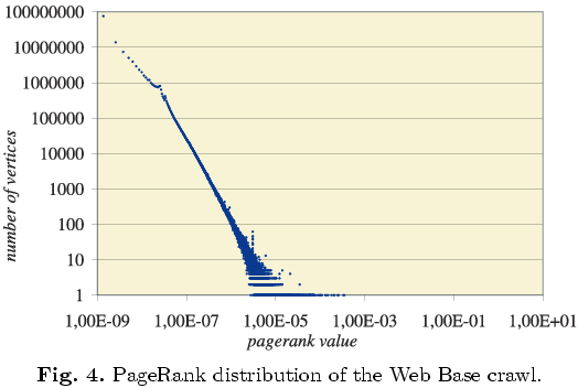
There are two problems with this kind of illustration. The first is parameter estimation: How did they estimate the parameters for the power-law distribution? The second is less obvious: Is it even appropriate to display PageRank values in such a way, and can you infer something about PageRank from this kind of diagram?
On the horizontal axis of this diagram, you have the PageRank values, and on the vertical axis, you have the number of vertices with this PageRank value. This kind of diagram is often used for degree distributions: You plot the vertex degree and the number of vertices with this degree on a doubly logarithmic scale, and if it comes out as a straight line, you have a power-law distribution.
The difference between degree distributions and a PageRank distribution is that degree distributions are discrete, but PageRank is a continous measure. There are not discrete “bins” in which to sort the vertices, according to their PageRank value. By counting how many vertices have a certain PageRank value, you implicitly discretize the values. What are the criteria for this discretization? The computational accuracy of your platform? The termination condition of your PageRank implementation? Some other discretization? Are the intervals of the same length, or do they have different length?
These questions are not addressed in the cited papers. Therefore, I tried to find a way to estimate the distribution of PageRank without using artificial discretization.
The diagram above is an example of a probability mass function. It is very easy to plot the probability mass function from a sample for a discrete distribution: You simply count the number of occurrences of the discrete values in your sample.
Unfortunately, there is no probability mass function for continuous distributions – because there is nothing to count. There is just the probability density function, which is much harder to estimate from a sample. Usually, you estimate the probability density function from a sample by using a kernel density estimator: You presume that each of your samples is generated by a normal distribution centered on the data point, with a fixed variance, and add up all those normal distributions to arrive at an estimate of the probability density function for the data set.
But kernel density estimation has two problems: It breaks down if the distribution very dissimilar to a normal distribution – for example a power-law distribution: The vast majority of data points for a power-law distribution will be at one extreme of the distribution, and a small number will be at the other extreme. But it is precisely this small number of data points we are interested in, since they determine (for example) the structure of the network. Kernel density estimation is prone to smooth over those data points. The second problem is that this gives you only an estimate of the density function, but it does not give you parameters for a density function in closed form. If you estimate those parameters from the estimated density function, you are estimating twice – with dismal prospects for the accuracy of your estimate.
Which brings us back to the original question: How do you estimate the parameters for a given probability distribution?
Basically, I know of three methods: a) a priori estimation, b) curve fitting, or c) using an estimator for the given distribution.
Method a) can be used to derive a distribution from a generating model for the given graph – for example, it can be used to prove that an Erdös-Renyi graph has a degree distribution following the Poisson distribution. However, my understanding of random graph processes and stochastics is not sufficient to go this route.
Method b) is what I used for estimating parameters of discrete probability distributions in my thesis: I plotted the probability mass function of the distribution and used non-linear least squares regression to fit the mass function of a known distribution (the Zeta distribution in my case) to my data points. While this is not a stochastically valid estimate, it worked well enough for my purposes.
In order to apply this method, I needed to find a suitable distribution, and a suitable representation of my sample to fit the distribution. A likely candidate for the distribution is the Pareto distribution, the continous counterpart to the Zeta distribution. I could not use the probability density function for estimating the parameters, because of the problems outlined above. But it is very easy to derive the cumulative distribution function for a sample of continous values – again by counting the number of data points below a certain threshold (thresholds can be set at each data point.)
A disadvantage of the cumulative distribution is that it is not as easy to see the power-law relationship as it is with the probability mass or density functions: For the density or mass function, you simply plot on a doubly-logarithmic scale, and if it is a straight line: power-law distribution. Therefore, the cumulative distribution is at a definitive disadvantage as regards the visual impact.
But it has the advantage that I do not have to estimate it, and that I can fit the cumulative distribution function of the Pareto distribution to it, using, again, non-linear least squares regression. Unfortunately, this did not give very good results: I could not find a set of parameters that fit this distribution well.
Therefore, method c) remains: Using an estimator for the distribution. For example, for the normal distribution, the sample mean is a maximum likelihood estimator for the mean of the distribution, and the sample variance is a maximum likelihood estimator for the variance.
For the Pareto distribution, a maximum likelihood estimator for the minimum possible value is the minimum of the sample. An estimator for the exponent is given in the article on the Pareto distribution cited above.
Using this method, I could find parameters for the Pareto distribution for my data set. The final estimate looked like this; the dashed line is the estimate, and the solid line is the real cumulative distribution. It is not a perfect fit, but it seems to go in the right direction:
![[cumulative distribution function]](/moebius/img/blog/prdistribution-0.png)
The maximum likelihood estimator seems to over-estimate the exponent; it puts the exponent at about 3.78. Using curve fitting, I got an even higher exponent: about 4.61, which is (visually at least) a worse estimate than the admittedly questionable one I derived with the maximum likelihood estimator.
For comparison, here is the estimated probability density function, along with a scatterplot of the data. It is rather useless for assessing the quality of the estimate, but it is visually pleasing, and gives a certain idea of the nature of the distribution:
![[probability density function]](/moebius/img/blog/prdistribution-1.png)
I cannot compare my results directly with the results cited above for the web graph, since I do not have the necessary dataset. I used a social network with about 1300 nodes – orders of magnitude smaller than the web graph, but it should follow a similar distribution. I do however hope that it is a valid method for estimating the parameters – and does not share the fundamental problem of treating PageRank as a discrete variable.
Two questions remain: Is the Pareto distribution really the distribution governing PageRank, or is there some other factor? And what would the results be for a larger graph – ideally the web graph? Would the quality of the estimate be better, or would it be worse? Do we perhaps have to look in a completely different direction for the distribution of PageRank?
UPDATE:Some further reading: Problems with fitting to the power-law distribution (Goldstein et.al., 2004), Estimators of the regression parameters of the zeta distribution (Doray, Arsenault, 2002), Power laws, Pareto distributions and Zipf’s law (Newman, 2005).
![[cover]](/moebius/books/charles_stross_the_atrocity_archives.large.jpg)